MNIST Variational Autoencoder
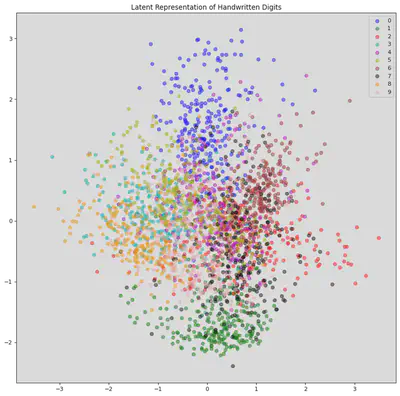
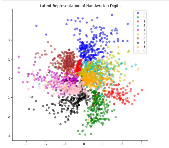 The latent space representation of the MNIST dataset.
The goal of a Variational Autoencoder is to create a generative model, such that we can call it and it will generate a sample that mimics the training dataset. Variational Autoencoders make the assumption that each of the samples $ \mathbf x_i$ from the data set $\mathbf{D}$ are iid and generated from the same probability distribution. Along with this, each sample has an latent feature vector $\mathbf{z}_i$. This implies the existence of a full joint distribution $p(\mathbf{x},\mathbf{z})$. When creating a generative model we are trying to discover the distribution $p(\mathbf x | \mathbf z)$, whereas when creating a discriminative model we are trying to discover the distribution $p(\mathbf{z}|\mathbf{x})$. VAEs are an attempt to utilize this latent structure to make optimization easier.
To start, let us first get our imports as well as our datset. For the purpose of this tutorial we will be using the MNIST dataset.
import matplotlib.pyplot as plt
import numpy as np
import torch as torch
import torchvision.datasets as datasets
from torchvision.transforms import ToTensor
from torch.utils.data import Dataset, DataLoader
import torch.nn as nn
import torch.nn.functional as F
import torch.optim as optim


class data(Dataset):

  def __init__(self, X, Y):
    self.X = X
    self.Y = Y
    if len(self.X) != len(self.Y):
      raise Exception("len(X) != len(Y)")

  def __len__(self):
    return len(self.X)

  def __getitem__(self, index):
    _x = self.X[index].unsqueeze(dim=0)
    _y = self.Y[index].unsqueeze(dim=0)

    return _x, _y

# Importing MNIST
mnist_trainset = datasets.MNIST(root='./data', train=True, download=True, transform=ToTensor())
mnist_testset = datasets.MNIST(root='./data', train=True, download=True, transform=ToTensor())

bs = 200

# Data Loader
train_loader = torch.utils.data.DataLoader(dataset=mnist_trainset, batch_size=bs, shuffle=True)
test_loader = torch.utils.data.DataLoader(dataset=mnist_testset, batch_size=bs, shuffle=False)
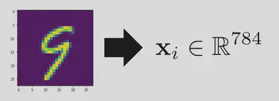
Lets consider what a particular sample from the dataset represents. We can take the image and then reshape it into a vector. Lets represent a particular sample by the symbol $\mathbf x_i$. We can represnt the probability of that element by assuming it is conditioned on some feature variable $\mathbf z_i$.
I am not interested in learning the distribution of $p(\mathbf x|\mathbf \phi)$ itself. Rather I want to know the conditionals $p(\mathbf x | \mathbf z, \mathbf \phi)$ and $p(\mathbf z| \mathbf x, \mathbf \phi)$. Where $\mathbf z$ is a “feature” space. This allows us to use the generative nature of $p(\mathbf x | \mathbf z, \mathbf \phi)$. We can choose a particular set of features $\mathbf z$ and then see which $\mathbf x$ probabilistically corresponds to it. Through all this we are then asserting that there exists a total joint distribution $p(\mathbf x, \mathbf z| \mathbf \phi)$. It is related to the conditionals through the following expression. Noting that $\mathbf \phi$ will represent the parameters of our model.
$$ p(\mathbf x|\mathbf \phi) = \int p(\mathbf{x},\mathbf{z}|\mathbf \phi) d\mathbf{z} $$
Sadly, I will be restricting our use of the actual image labels in MNIST. This is to make this more generic to image generation in general. We only have observed samples from $p(\mathbf x|\mathbf \phi)$. We can then write the objection fuction using a maximum likelihood treatment as:
$$ \log p(\mathbf x|\mathbf \phi) = \log \bigg[\int p(\mathbf{x},\mathbf{z}|\mathbf \phi) d\mathbf{z}\bigg] $$
Sadly the integral in the equation above makes it quite difficult to deal with. Therefore, we can instead make an approximate model for this system by using two neural networks. One of these networks will be the encoder, the $p(\mathbf x|\mathbf \phi)$ that we have seen thus far, and the other will be a decoder. I am going to use the function $q(\mathbf x |\mathbf z, \mathbf \theta)$ to represent the decoder where $\mathbf \theta$ are the network parameters. Similarly, the decoder will be $q(\mathbf z |\mathbf x, \mathbf \theta)$.
$$ \mathbf \mu, \mathbf \Sigma = \text{Encoder}_\theta(\mathbf x) $$ $$ q(\mathbf z |\mathbf x, \mathbf \theta) = \mathcal{N}(\mathbf z | \mathbf \mu, \mathbf \Sigma) $$
Then notice that we can write the objective function can then be written as:
$$ \log p(\mathbf x |\mathbf \phi) = \mathbb{E}_{q(\mathbf z |\mathbf x, \mathbf \theta)}[\log p(\mathbf x |\mathbf \phi)] $$
Because the integral introduced by the expectation doesn’t depend on $\mathbb x$ we can just take it out and let $q(\mathbf z |\mathbf x, \mathbf \theta)$ integrate itself to 1. This expression alows for more decomposition.
$$ \mathbb{E}_{q(\mathbf z |\mathbf x, \mathbf \theta)}\bigg[\log p(\mathbf x |\mathbf \phi)\bigg] $$
$$ = \mathbb{E}_{q(\mathbf z |\mathbf x, \mathbf \theta)}\bigg[\log\bigg( \frac{p(\mathbf x,\mathbf z |\mathbf \phi) }{p(\mathbf z|\mathbf \phi,\mathbf x)}\bigg) \bigg] $$
This is because the marginalized probability can be written in terms of the joint and a conditional. Further then we can simply multiply the top and bottom by the same quantitiy and separate the logarithm into a sum.
$$ = \mathbb{E}_{q(\mathbf z |\mathbf x, \mathbf \theta)}\bigg[\log\bigg( \frac{p(\mathbf x,\mathbf z|\mathbf \phi)q(\mathbf z |\mathbf x, \mathbf \theta)}{p(\mathbf z|\mathbf \phi, \mathbf x)q(\mathbf z |\mathbf x, \mathbf \theta)}\bigg) \bigg] $$ . $$ = \mathbb{E}_{q(\mathbf z |\mathbf x, \mathbf \theta)}\bigg[\log\bigg( \frac{p(\mathbf x,\mathbf z|\mathbf \phi)}{q(\mathbf z |\mathbf x, \mathbf \theta)}\bigg) \bigg] + \mathbb{E}_{q(\mathbf z |\mathbf x, \mathbf \theta)}\bigg[\log\bigg( \frac{q(\mathbf z |\mathbf x, \mathbf \theta)}{p(\mathbf z|\mathbf \phi, \mathbf x)}\bigg) \bigg] $$
We can recognize the second expectation as the KL divergence between our network model and the true distribution. The KL divergence is strictly positive, therefore we can view the first expectation as an evidence based lower bound (ELBO) of the true likelihood of the data. If we maximize the lower bound we will be also maximizing the probaility of the data. This totally reframes the problem of inference.
$$ \text{ELBO} = \mathbb{E}_{q(\mathbf z |\mathbf x, \mathbf \theta)}\bigg[\log\bigg( \frac{p(\mathbf x,\mathbf z)}{q(\mathbf z |\mathbf x, \mathbf \theta)}\bigg) \bigg] $$ $$ = \mathbb{E}_{q(\mathbf z |\mathbf x, \mathbf \theta)}\bigg[\log p(\mathbf x,\mathbf z) \bigg] - \mathbb{E}_{q(\mathbf z |\mathbf x, \mathbf \theta)}\bigg[\log q(\mathbf z |\mathbf x, \mathbf \theta)\bigg] \ $$ $$ = \mathbb{E}_{q(\mathbf z |\mathbf x, \mathbf \theta)}\bigg[\log p(\mathbf x| \mathbf z, \mathbf \phi)p(\mathbf z) \bigg] - \mathbb{E}_{q(\mathbf z |\mathbf x, \mathbf \theta)}\bigg[\log q(\mathbf z |\mathbf x, \mathbf \theta)\bigg] \ $$
We can then take $p(\mathbf z)$ as a prior distribution of our data. Let us choose that as a standard normal $\mathcal{N}(\mathbf z | \mathbf \mu = \mathbf 0, \mathbf \Sigma = \mathbf I)$. This lets us write our expression out as follows:
$$ \mathbb{E}_{q(\mathbf z |\mathbf x, \mathbf \theta)}\bigg[\log p(\mathbf x| \mathbf z, \mathbf \phi)\bigg] + \mathbb{E}_{q(\mathbf z |\mathbf x, \mathbf \theta)}\bigg[\log p(\mathbf z)\bigg] - \mathbb{E}_{q(\mathbf z |\mathbf x, \mathbf \theta)}\bigg[\log q(\mathbf z |\mathbf x, \mathbf \theta)\bigg] \ $$
$$ = \mathbb{E}_{q(\mathbf z |\mathbf x, \mathbf \theta)}\bigg[\log p(\mathbf x| \mathbf z, \mathbf \phi)\bigg] + \mathbb{E}_{q(\mathbf z |\mathbf x, \mathbf \theta)}\bigg[\log( p(\mathbf z)/q(\mathbf z |\mathbf x, \mathbf \theta))\bigg] $$
Then the second term corresponds to the negative KL divergence between the prior and our model. Remeber we asserted $q(\mathbf z |\mathbf x, \mathbf \theta)$ is normal. Making that part of the expression quite simple. We can then assert that the generative distribution is also gaussian. We can choose our network to just calculate the mean value. This makes the probability of a training set become the MSE loss.
recon_error = nn.MSELoss(reduction='sum')
def variational_loss(p_x,x,μ_qz,log_var_qz,ϵ,z):
    KL = -0.5 * torch.sum(log_var_qz - μ_qz.pow(2) - log_var_qz.exp()) # - KL Divergece between standard normal and current p(z) and q(z|x)
    return recon_error(p_x,x) + KL
Now we need to discuss backpropigation within this network. When we are computing our loss function, it has to be taken as the expecation with respect to $q(\mathbf z |\mathbf x, \mathbf \theta)$. This means we must use a monte carlo estimate to evaluate the expectation as the integral is intractable. However this makes backpropigation impossible, we cant backprop through a random variable. Therefore we may reparameterize the randomness into some dummy variable $\epsilon$. Because our distribution is gaussian, we may simply choose $\epsilon$ as a standard normal and use the network output to rescale it. As for the network, we will keep it simple and just do three layers for the encoder and 3 for the deconder. See the implementation below.
class VAE(nn.Module):

    def __init__(self):
        super(VAE,self).__init__()

        # define encoder layers
        self.e_dense1 = nn.Linear(784,64)
        self.e_dense2 = nn.Linear(64, 32)
        self.e_dense3 = nn.Linear(32, 8)

        # define dencoder layers
        self.d_dense1 = nn.Linear(4,32)
        self.d_dense2 = nn.Linear(32, 64)
        self.d_dense3 = nn.Linear(64, 784)


    def encode(self, x):
        x = torch.relu(self.e_dense1(x))
        x = torch.relu(self.e_dense2(x))
        x = (self.e_dense3(x))
        return x[:,:4],x[:,4:]

    def sample(self,μ,log_var):
        σ = torch.exp(0.5*log_var)
        ϵ = torch.randn_like(σ) # Sample from epsilon
        return μ + ϵ.mul(σ),ϵ # transform epsilon into z sample

    def decode(self, x):
        x = torch.relu(self.d_dense1(x))
        x = torch.relu(self.d_dense2(x))
        x = torch.sigmoid(self.d_dense3(x))
        return x

    def forward(self,x):
        μ_qz,log_var_qz = self.encode(x)
        z,ϵ = self.sample(μ_qz,log_var_qz)
        p_x = self.decode(z)
        return p_x,μ_qz,log_var_qz,ϵ,z
Now we can instantiate our model and run it!!
vae = VAE()
optimizer = optim.Adam(vae.parameters())
criterion = variational_loss
for epoch in range(50): # loop over the dataset multiple times
total_loss = 0.0
for i, data in enumerate(train_loader,start = 1):
inputs = data[0].flatten(start_dim=1)
# zero the parameter gradients
optimizer.zero_grad()
# forward + backward + optimize
p_x,μ_qz,log_var_qz,ϵ,z = vae(inputs)
loss = criterion(p_x,inputs,μ_qz,log_var_qz,ϵ,z)
loss.backward()
optimizer.step()
total_loss += loss.item()
if i % 100 == 0:
print('Epoch: {} [{}/{} ({:.0f}%)]\tLoss: {:.6f}'.format(
epoch, i * len(inputs), len(train_loader.dataset),
(100*(len(inputs) * i) / len(train_loader.dataset)), loss.item() / len(inputs)))
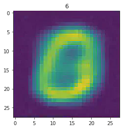
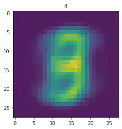
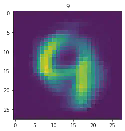
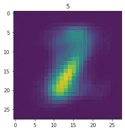
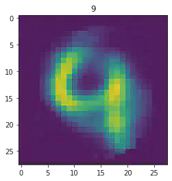
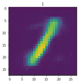
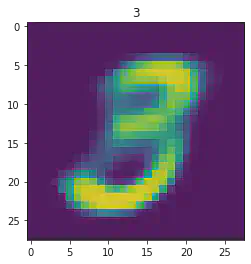
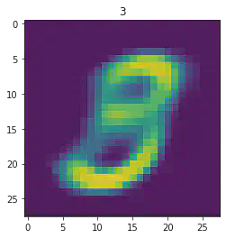
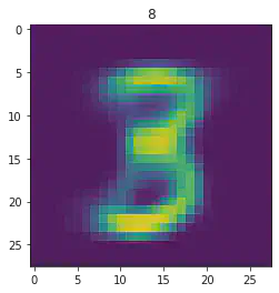
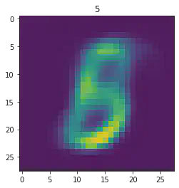
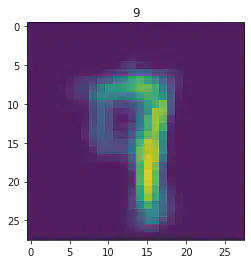
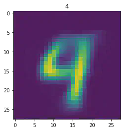
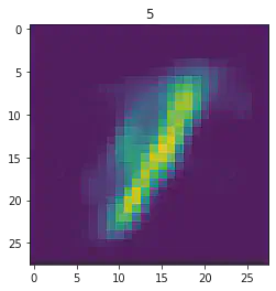
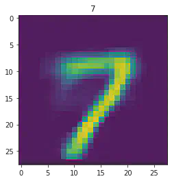
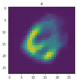
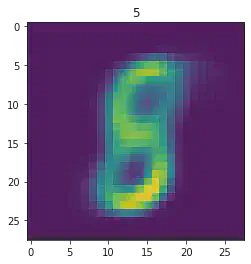
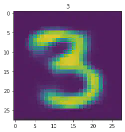
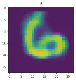
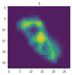
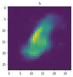
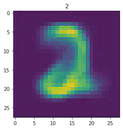
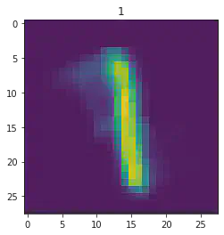
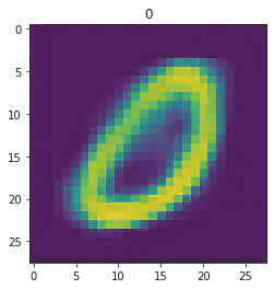
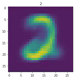
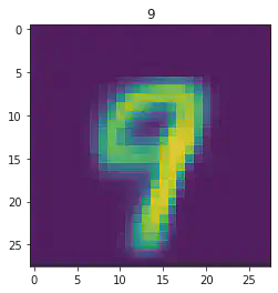
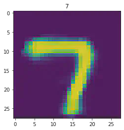
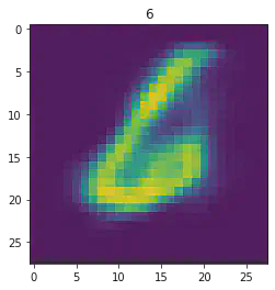
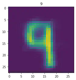
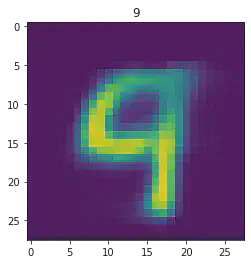
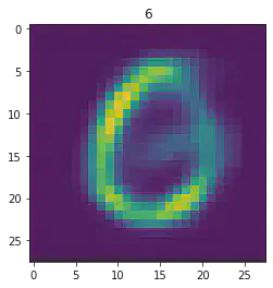
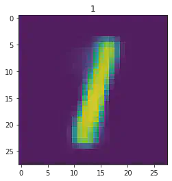
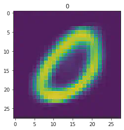
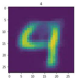
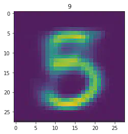
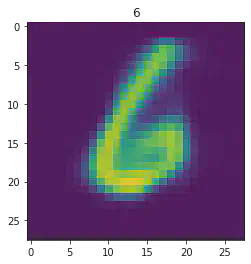
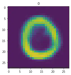
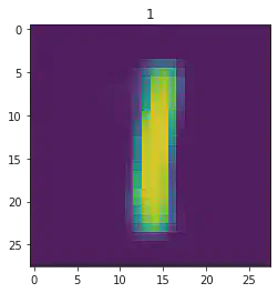
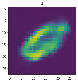
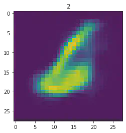
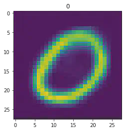
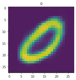
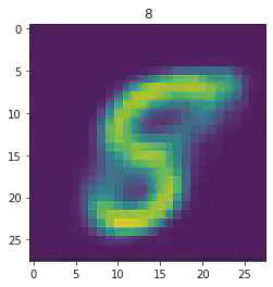
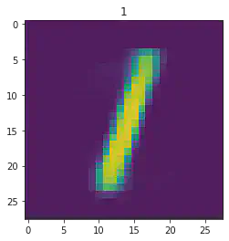
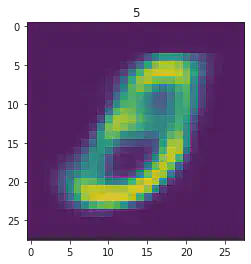
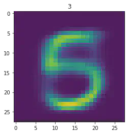
sample_idx = np.random.randint(len(mnist_trainset))
μ,σ = vae.encode(torch.stack((mnist_trainset[sample_idx][0].flatten(),mnist_trainset[sample_idx][0].flatten())))
z,ϵ = vae.sample(μ,σ)
x = vae.decode(z.unsqueeze(dim=1))
plt.imshow(x[1].detach().numpy().reshape(28,28))
plt.title(mnist_trainset[sample_idx][1])
plt.show()
print('====> Epoch: {} Average loss: {:.4f}'.format(epoch, total_loss / len(train_loader.dataset)))
print('Finished Training')
Epoch: 0 [20000/60000 (33%)]	Loss: 56.698457
Epoch: 0 [40000/60000 (67%)]	Loss: 54.966836
Epoch: 0 [60000/60000 (100%)]	Loss: 53.562334
====> Epoch: 0 Average loss: 66.2929
Epoch: 1 [20000/60000 (33%)]	Loss: 51.518516
Epoch: 1 [40000/60000 (67%)]	Loss: 50.127305
Epoch: 1 [60000/60000 (100%)]	Loss: 47.599878
====> Epoch: 1 Average loss: 50.3971
Epoch: 2 [20000/60000 (33%)]	Loss: 46.609116
Epoch: 2 [40000/60000 (67%)]	Loss: 44.889531
Epoch: 2 [60000/60000 (100%)]	Loss: 43.474600
====> Epoch: 2 Average loss: 46.2344
Epoch: 3 [20000/60000 (33%)]	Loss: 42.524268
Epoch: 3 [40000/60000 (67%)]	Loss: 41.891636
Epoch: 3 [60000/60000 (100%)]	Loss: 41.541118
====> Epoch: 3 Average loss: 42.6844
Epoch: 4 [20000/60000 (33%)]	Loss: 41.212432
Epoch: 4 [40000/60000 (67%)]	Loss: 40.988394
Epoch: 4 [60000/60000 (100%)]	Loss: 40.674072
====> Epoch: 4 Average loss: 41.3674
Epoch: 5 [20000/60000 (33%)]	Loss: 39.347095
Epoch: 5 [40000/60000 (67%)]	Loss: 39.964746
Epoch: 5 [60000/60000 (100%)]	Loss: 39.661968
====> Epoch: 5 Average loss: 40.5180
Epoch: 6 [20000/60000 (33%)]	Loss: 39.077688
Epoch: 6 [40000/60000 (67%)]	Loss: 38.294802
Epoch: 6 [60000/60000 (100%)]	Loss: 38.347146
====> Epoch: 6 Average loss: 39.9005
Epoch: 7 [20000/60000 (33%)]	Loss: 40.272634
Epoch: 7 [40000/60000 (67%)]	Loss: 39.569946
Epoch: 7 [60000/60000 (100%)]	Loss: 38.919097
====> Epoch: 7 Average loss: 39.3812
Epoch: 8 [20000/60000 (33%)]	Loss: 38.082427
Epoch: 8 [40000/60000 (67%)]	Loss: 38.717292
Epoch: 8 [60000/60000 (100%)]	Loss: 37.672859
====> Epoch: 8 Average loss: 38.9434
Epoch: 9 [20000/60000 (33%)]	Loss: 37.330728
Epoch: 9 [40000/60000 (67%)]	Loss: 37.700049
Epoch: 9 [60000/60000 (100%)]	Loss: 37.563271
====> Epoch: 9 Average loss: 38.5736
Epoch: 10 [20000/60000 (33%)]	Loss: 37.702485
Epoch: 10 [40000/60000 (67%)]	Loss: 38.086489
Epoch: 10 [60000/60000 (100%)]	Loss: 37.647063
====> Epoch: 10 Average loss: 38.2347
Epoch: 11 [20000/60000 (33%)]	Loss: 37.480168
Epoch: 11 [40000/60000 (67%)]	Loss: 36.328479
Epoch: 11 [60000/60000 (100%)]	Loss: 37.478169
====> Epoch: 11 Average loss: 37.9565
Epoch: 12 [20000/60000 (33%)]	Loss: 37.965278
Epoch: 12 [40000/60000 (67%)]	Loss: 38.572202
Epoch: 12 [60000/60000 (100%)]	Loss: 36.891362
====> Epoch: 12 Average loss: 37.7104
Epoch: 13 [20000/60000 (33%)]	Loss: 37.276660
Epoch: 13 [40000/60000 (67%)]	Loss: 37.544507
Epoch: 13 [60000/60000 (100%)]	Loss: 36.613884
====> Epoch: 13 Average loss: 37.5024
Epoch: 14 [20000/60000 (33%)]	Loss: 37.619067
Epoch: 14 [40000/60000 (67%)]	Loss: 37.133477
Epoch: 14 [60000/60000 (100%)]	Loss: 37.386440
====> Epoch: 14 Average loss: 37.3065
Epoch: 15 [20000/60000 (33%)]	Loss: 37.111313
Epoch: 15 [40000/60000 (67%)]	Loss: 37.020078
Epoch: 15 [60000/60000 (100%)]	Loss: 37.991951
====> Epoch: 15 Average loss: 37.1374
Epoch: 16 [20000/60000 (33%)]	Loss: 36.601738
Epoch: 16 [40000/60000 (67%)]	Loss: 36.642373
Epoch: 16 [60000/60000 (100%)]	Loss: 36.532485
====> Epoch: 16 Average loss: 36.9795
Epoch: 17 [20000/60000 (33%)]	Loss: 37.645845
Epoch: 17 [40000/60000 (67%)]	Loss: 38.491716
Epoch: 17 [60000/60000 (100%)]	Loss: 36.673926
====> Epoch: 17 Average loss: 36.8425
Epoch: 18 [20000/60000 (33%)]	Loss: 36.183394
Epoch: 18 [40000/60000 (67%)]	Loss: 36.757959
Epoch: 18 [60000/60000 (100%)]	Loss: 37.720042
====> Epoch: 18 Average loss: 36.7152
Epoch: 19 [20000/60000 (33%)]	Loss: 36.210232
Epoch: 19 [40000/60000 (67%)]	Loss: 37.483999
Epoch: 19 [60000/60000 (100%)]	Loss: 36.998501
====> Epoch: 19 Average loss: 36.5916
Epoch: 20 [20000/60000 (33%)]	Loss: 36.686836
Epoch: 20 [40000/60000 (67%)]	Loss: 36.176907
Epoch: 20 [60000/60000 (100%)]	Loss: 37.291575
====> Epoch: 20 Average loss: 36.4815
Epoch: 21 [20000/60000 (33%)]	Loss: 35.280510
Epoch: 21 [40000/60000 (67%)]	Loss: 35.408699
Epoch: 21 [60000/60000 (100%)]	Loss: 36.384626
====> Epoch: 21 Average loss: 36.3850
Epoch: 22 [20000/60000 (33%)]	Loss: 36.342734
Epoch: 22 [40000/60000 (67%)]	Loss: 36.120286
Epoch: 22 [60000/60000 (100%)]	Loss: 34.955454
====> Epoch: 22 Average loss: 36.2792
Epoch: 23 [20000/60000 (33%)]	Loss: 35.759111
Epoch: 23 [40000/60000 (67%)]	Loss: 34.986384
Epoch: 23 [60000/60000 (100%)]	Loss: 35.863618
====> Epoch: 23 Average loss: 36.2050
Epoch: 24 [20000/60000 (33%)]	Loss: 35.652568
Epoch: 24 [40000/60000 (67%)]	Loss: 37.206226
Epoch: 24 [60000/60000 (100%)]	Loss: 37.563311
====> Epoch: 24 Average loss: 36.1336
Epoch: 25 [20000/60000 (33%)]	Loss: 37.236667
Epoch: 25 [40000/60000 (67%)]	Loss: 36.156731
Epoch: 25 [60000/60000 (100%)]	Loss: 34.020962
====> Epoch: 25 Average loss: 36.0415
Epoch: 26 [20000/60000 (33%)]	Loss: 35.965017
Epoch: 26 [40000/60000 (67%)]	Loss: 36.913325
Epoch: 26 [60000/60000 (100%)]	Loss: 35.093923
====> Epoch: 26 Average loss: 35.9669
Epoch: 27 [20000/60000 (33%)]	Loss: 35.891963
Epoch: 27 [40000/60000 (67%)]	Loss: 36.001890
Epoch: 27 [60000/60000 (100%)]	Loss: 36.545264
====> Epoch: 27 Average loss: 35.8938
Epoch: 28 [20000/60000 (33%)]	Loss: 37.059600
Epoch: 28 [40000/60000 (67%)]	Loss: 35.631221
Epoch: 28 [60000/60000 (100%)]	Loss: 35.151846
====> Epoch: 28 Average loss: 35.8239
Epoch: 29 [20000/60000 (33%)]	Loss: 35.101321
Epoch: 29 [40000/60000 (67%)]	Loss: 34.398643
Epoch: 29 [60000/60000 (100%)]	Loss: 34.386650
====> Epoch: 29 Average loss: 35.7588
Epoch: 30 [20000/60000 (33%)]	Loss: 35.678657
Epoch: 30 [40000/60000 (67%)]	Loss: 35.820137
Epoch: 30 [60000/60000 (100%)]	Loss: 35.145249
====> Epoch: 30 Average loss: 35.7031
Epoch: 31 [20000/60000 (33%)]	Loss: 34.647329
Epoch: 31 [40000/60000 (67%)]	Loss: 34.748079
Epoch: 31 [60000/60000 (100%)]	Loss: 35.683723
====> Epoch: 31 Average loss: 35.6446
Epoch: 32 [20000/60000 (33%)]	Loss: 35.611414
Epoch: 32 [40000/60000 (67%)]	Loss: 37.895881
Epoch: 32 [60000/60000 (100%)]	Loss: 35.952639
====> Epoch: 32 Average loss: 35.5910
Epoch: 33 [20000/60000 (33%)]	Loss: 36.365115
Epoch: 33 [40000/60000 (67%)]	Loss: 33.621260
Epoch: 33 [60000/60000 (100%)]	Loss: 36.825591
====> Epoch: 33 Average loss: 35.5494
Epoch: 34 [20000/60000 (33%)]	Loss: 36.096372
Epoch: 34 [40000/60000 (67%)]	Loss: 36.678503
Epoch: 34 [60000/60000 (100%)]	Loss: 34.051584
====> Epoch: 34 Average loss: 35.4977
Epoch: 35 [20000/60000 (33%)]	Loss: 34.831150
Epoch: 35 [40000/60000 (67%)]	Loss: 35.734529
Epoch: 35 [60000/60000 (100%)]	Loss: 34.864536
====> Epoch: 35 Average loss: 35.4564
Epoch: 36 [20000/60000 (33%)]	Loss: 35.273062
Epoch: 36 [40000/60000 (67%)]	Loss: 36.339285
Epoch: 36 [60000/60000 (100%)]	Loss: 35.096025
====> Epoch: 36 Average loss: 35.4226
Epoch: 37 [20000/60000 (33%)]	Loss: 35.747583
Epoch: 37 [40000/60000 (67%)]	Loss: 34.885400
Epoch: 37 [60000/60000 (100%)]	Loss: 35.150825
====> Epoch: 37 Average loss: 35.3787
Epoch: 38 [20000/60000 (33%)]	Loss: 35.365684
Epoch: 38 [40000/60000 (67%)]	Loss: 35.076494
Epoch: 38 [60000/60000 (100%)]	Loss: 35.274106
====> Epoch: 38 Average loss: 35.3375
Epoch: 39 [20000/60000 (33%)]	Loss: 33.656929
Epoch: 39 [40000/60000 (67%)]	Loss: 34.410693
Epoch: 39 [60000/60000 (100%)]	Loss: 35.632637
====> Epoch: 39 Average loss: 35.3154
Epoch: 40 [20000/60000 (33%)]	Loss: 35.789722
Epoch: 40 [40000/60000 (67%)]	Loss: 36.411433
Epoch: 40 [60000/60000 (100%)]	Loss: 36.640859
====> Epoch: 40 Average loss: 35.2726
Epoch: 41 [20000/60000 (33%)]	Loss: 36.135540
Epoch: 41 [40000/60000 (67%)]	Loss: 33.705623
Epoch: 41 [60000/60000 (100%)]	Loss: 36.202119
====> Epoch: 41 Average loss: 35.2119
Epoch: 42 [20000/60000 (33%)]	Loss: 35.541836
Epoch: 42 [40000/60000 (67%)]	Loss: 35.629856
Epoch: 42 [60000/60000 (100%)]	Loss: 34.619102
====> Epoch: 42 Average loss: 35.1965
Epoch: 43 [20000/60000 (33%)]	Loss: 35.975867
Epoch: 43 [40000/60000 (67%)]	Loss: 34.694214
Epoch: 43 [60000/60000 (100%)]	Loss: 34.779368
====> Epoch: 43 Average loss: 35.1655
Epoch: 44 [20000/60000 (33%)]	Loss: 34.862920
Epoch: 44 [40000/60000 (67%)]	Loss: 35.202686
Epoch: 44 [60000/60000 (100%)]	Loss: 35.154026
====> Epoch: 44 Average loss: 35.1412
Epoch: 45 [20000/60000 (33%)]	Loss: 35.493105
Epoch: 45 [40000/60000 (67%)]	Loss: 34.763962
Epoch: 45 [60000/60000 (100%)]	Loss: 36.250828
====> Epoch: 45 Average loss: 35.1256
Epoch: 46 [20000/60000 (33%)]	Loss: 35.688271
Epoch: 46 [40000/60000 (67%)]	Loss: 36.289146
Epoch: 46 [60000/60000 (100%)]	Loss: 35.851013
====> Epoch: 46 Average loss: 35.0912
Epoch: 47 [20000/60000 (33%)]	Loss: 34.039561
Epoch: 47 [40000/60000 (67%)]	Loss: 36.419995
Epoch: 47 [60000/60000 (100%)]	Loss: 34.943896
====> Epoch: 47 Average loss: 35.0557
Epoch: 48 [20000/60000 (33%)]	Loss: 33.076106
Epoch: 48 [40000/60000 (67%)]	Loss: 36.028267
Epoch: 48 [60000/60000 (100%)]	Loss: 35.647769
====> Epoch: 48 Average loss: 35.0177
Epoch: 49 [20000/60000 (33%)]	Loss: 36.092920
Epoch: 49 [40000/60000 (67%)]	Loss: 36.263647
Epoch: 49 [60000/60000 (100%)]	Loss: 34.410708
====> Epoch: 49 Average loss: 35.0090
Finished Training
We can visualize the latent space by evaluating the training samples and then save the resulting mean value for $\mathbf z$
Zx = [[] for i in range(10)]
Zy = [[] for i in range(10)]
for i in range(len(mnist_trainset)):
    μ,σ = vae.encode(torch.stack((mnist_trainset[i][0].flatten(),mnist_trainset[i][0].flatten())))
    Zx[mnist_trainset[i][1]].append(μ[0].detach().numpy()[0])
    Zy[mnist_trainset[i][1]].append(μ[0].detach().numpy()[1])
fig = plt.figure(figsize=(12, 12),dpi=80)

ax = fig.add_subplot()
N = 250

C = ['b','g','r','c','m','y','brown','black','orange','pink']
for i in range(10):
    ax.scatter(Zx[i][:N],Zy[i][:N],label=i,alpha=0.5,color=C[i])

for i in range(0,10,-1):
    plt.scatter(Zx[i][N:2*N],Zy[i][N:2*N],label=i,alpha=0.5,color=C[i])

plt.legend()
plt.title("Latent Representation of Handwritten Digits")
plt.show()
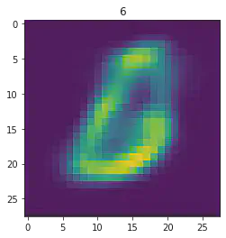
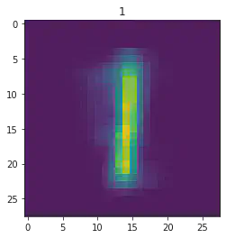
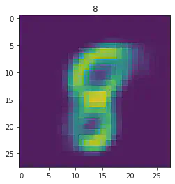
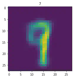
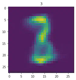
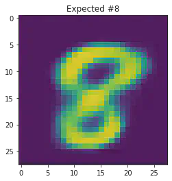
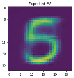
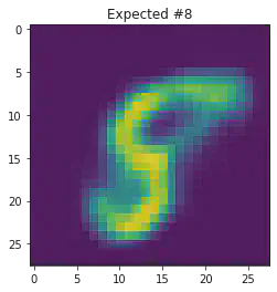
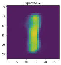
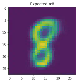
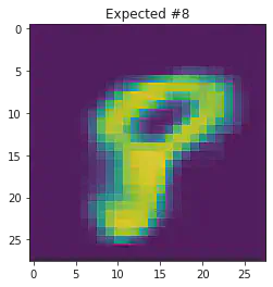
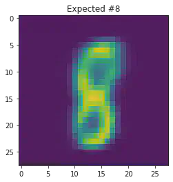
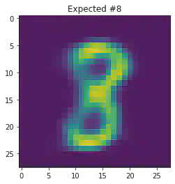
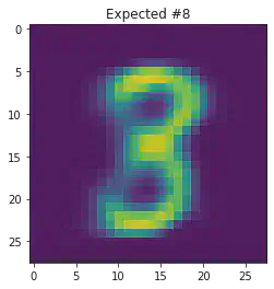
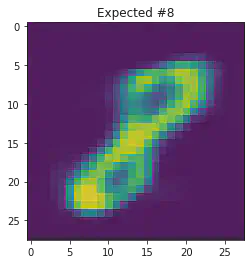
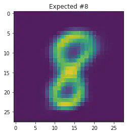
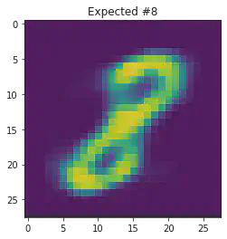
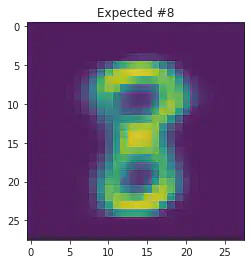
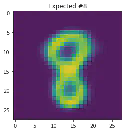
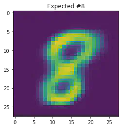
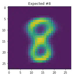
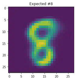
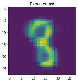
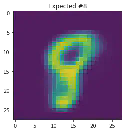
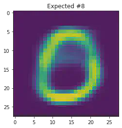
We can also use this to to see how well it will produce a handwritten digit with a specified label.
for i in range(20):

    sample_idx = np.random.randint(len(mnist_trainset))
    while (mnist_trainset[sample_idx][1]) != 8:
        sample_idx = np.random.randint(len(mnist_trainset))

    μ,σ = vae.encode(torch.stack((mnist_trainset[sample_idx][0].flatten(),mnist_trainset[sample_idx][0].flatten())))
    z,ϵ = vae.sample(μ,σ)
    x = vae.decode(z.unsqueeze(dim=1))
    plt.imshow(x[1].detach().numpy().reshape(28,28))
    plt.title("Expected #"+ str(mnist_trainset[sample_idx][1]))
    plt.show()
Sources:
- https://arxiv.org/pdf/1906.02691.pdf
- Bishop Pattern Recognition and Machine Learning
- Wikipedia
Harry Winston Sullivan
PhD Student and Bayesian Bro
Mathematics, the only hobby which somehow makes you both smarter and stupider at the same time. There is too many things to read and not enough time to do so.